User Manual of HIBLUP

1.1.What is HIBLUP
HIBLUP (say “Hi!” to BLUP), which is called “天权”in Chinese, is an user-friendly software that provides estimated genetic value of each individual by maximizing the usage of information from pedigree, genome, and phenotype, as well as all process-related functions, such as construction of relationship matrix, estimation of variance components (heritability) of traits and co-variance components (genetic correlation) between traits using various algorithms, solution of mixed model, computation of SNP effects, and implement of genomic mating. Users can easily achieve simple linear model (LM), best linear unbiased predictors (BLUP), pedigree basedBLUP (PBLUP), genomic BLUP (GBLUP), and single-step GBLUP (SSGBLUP) for single trait model, repeated traits model, and multiple traits model. The functions of HIBLUP will keep on being enriched with more functionalities based on users feedback.
1.2.Where to download HIBLUP
The latest released executable file of HIBLUP for different platforms can be downloaded from:
https://www.hiblup.com/download.
It is free of charge for academic purposes. For commercial purposes, please contact the development team.
1.3.How to cite HIBLUP
For the HIBLUP Software, please cite:
Lilin Yin#, Haohao Zhang#, Zhenshuang Tang, Dong Yin, Yuhua Fu, Xiaohui Yuan, Xinyun Li*, Xiaolei Liu*, Shuhong Zhao*. “HIBLUP: an integration of statistical models on the BLUP framework for efficient genetic evaluation using big genomic data” Nucleic Acids Research (2023): gkad074.
For genomic mating, please cite:
Zhenshuang# Tang, Lilin Yin#, Dong Yin, Haohao Zhang, Yuhua Fu, Guangliang Zhou, Yunxiang Zhao, Zhiquan Wang, Xiaolei Liu*, Xinyun Li*, Shuhong Zhao*. “Development and application of an efficient genomic mating method to maximize the production performances of three-way crossbred pigs.” Briefings in Bioinformatics 24.1 (2023): bbac587.
1.4.Contact us
HIBLUP is developed at Zhao lab of Huazhong Agricultural University.
Design and Maintenance team:
Lilin Yin#, Haohao Zhang#, Zhenshuang Tang, Dong Yin, Yuhua Fu, Xiaohui Yuan, Xinyun Li*, Xiaolei Liu*, Shuhong Zhao*
Questions, suggestions, and bug reports are welcome and appreciated, we recommend sending your message by filling the form in the following page:
https://www.hiblup.com/contact-us
If it cannot fully express your question or you get a trouble from the above page, please feel free to send us email by:
Lilin Yin (尹立林): ylilin@mail.hzau.edu.cn
HaoHao Zhang (张浩浩): haohaozhang@whut.edu.cn
Xiaolei Liu (刘小磊): xiaoleiliu@mail.hzau.edu.cn
2.Input File Formats
2.1.Phenotype file
Different with other software, the phenotype file required for HIBLUP should include not only the phenotypic records, but also the environmental covariates, fixed and random effects. The first column must be the individual id, header should be included in the file. Brief view of example phenotype file is as follows:
id	sex	season	day	weight	loc	dam	tr1	tr2	tr3
Ind1	F	Winter	100	2.9	l3	Ind902	73.9776	21.3252	35.7737
Ind2	M	Summer	100	1.5	l2	Ind902	94.1994	19.1162	54.2453
Ind3	M	Winter	100	1.8	l4	Ind903	88.6698	5.9538	71.0284
Ind4	M	Winter	100	1.9	l1	Ind903	87.0458	-2.8179	37.2703
Ind5	M	Spring	100	2.2	l3	Ind905	68.8077	2.5357	59.5402
Ind6	F	Autumn	100	1.9	l1	Ind905	85.9242	-3.06	48.4822
Any symbol below will be treated as missing when loading the file:
NA Na . - NaN NAN nan na N/A n/a <NA>
The file should be assigned to the parametric option --pheno.
By default, HIBLUP will take the trait at second column for analysis, users can specify a different column by using --pheno-pos n, for example, --pheno-pos 8 represents using the 8th column for analysis.
NOTE
If there are multiple traits to be used for estimating genetic correlation, please use space as separator, e.g. --pheno-pos 8 9 10.
2.2.Covariates, fixed and environmental random effects
For covariates, fixed effect and environmental random effect of a trait, please specify its position at phenotype file to flag --qcovar, --dcovar, --rand respectively.
For single trait, please use comma as separator, for example:--qcovar 4,5: take “day” and “weight” as covariates--dcovar 2,3: take “sex” and “season” as fixed effects--rand 6: take “loc” as environmental random effect
For multiple traits, if there are some environmental factors needed to be fitted as a model effect, all traits should be specified at this model effect, and please use comma as separator within a trait, and use space among traits, use 0 for a trait if those factors are not considered for it, take fixed effect for an example:
./hiblup ... --dcovar 2,3 0 2,3,6 ...
which means there are 3 traits in analysis, the first trait has two fixed effects: “sex” and “season“; the second trait has no fixed effect; the third trait has three fixed effects, which are “sex“, “season” and “loc“.
IMPORTANT
--qcovar is used to specify the environmental effects as quantitative covariates, the records for the effects should be in digits, any character is not allowed.
--dcovar is used to specify the environmental effects as discrete covariates, the records for the effects could be in either digits or characters, both are acceptable.
--rand is used to specify the environmental random effects, which come from the recorded environmental factors, the genetic random effects are from either pedigree or genomic information, if pedigree or genotype file is provided, HIBLUP will fit the genetic random effect in the model automatically, users DO NOT need to add the column of individuals id as random effect here.
2.3.Pedigree file
Pedigree file is used for deriving numerator relationship matrix and inbreeding coefficient. Three columns in file are required orderly. The first column is the individual id, the second and third columns are its father and mother id respectively.
NA Na . - NaN NAN nan na N/A n/a <NA>
As the same with phenotype file, any symbol of the list above appears in the pedigree file will be treated as missing. An example file for pedigree is as following:
id	father	mother
Ind2	NA	NA
Ind5	Ind1	NA
Ind11	NA	Ind2
Ind17	Ind11	Ind5
Ind22	Ind1	Ind5
Ind45	Ind22	Ind2
The file should be assigned to flag --pedigree.
NOTE
The order of individual id in the first column can be ranked by birth date, but it is not a compulsive requirement, as HIBLUP has the automatic function of sorting and rearrangement on the input pedigree.
2.4.Genotype file
HIBLUP currently only accept the genotype in PLINK binary format, e.g. demo.fam, demo.bim and demo.bed, please see more details about these files at PLINK user manual. Users can convert any other format of genotype (e.g. VCF, HapMap, PED/MAP) to binary format by PLINK2 and TASSEL:
# HapMap to VCF by TASSEL
./run_pipeline.pl -SortGenotypeFilePlugin -inputFile demo.hmp.txt
                  -outputFile demo.sort.hmp.txt -fileType Hapmap
./run_pipeline.pl -fork1 -h demo.sort.hmp.txt -export-exportType VCF -runfork1
# VCF to Binary
./plink2 --vcf demo.vcf --make-bed --out demo
# PED/MAP to Binary
./plink2 --ped demo.ped --map demo.map --make-bed --out demo
These binary files should be assigned to parametric option --bfile [prefix] (i.e., --bfile demo)
NOTE
(1) HIBLUP only supports to load one binary file, does not support to load more than one binary files (e.g., whole genome is stored separately by chromosome), please merge them by PLINK prior to using HIBLUP, a rough guidance can be found here.
(2) HIBLUP will code the genotype A1A1 as 2, A1A2 as 1, and A2A2 as 0, where A1 is the first allele of each marker in *.bim file, therefore the estimated effect size is on A1 allele, users should pay attention to it when a process involves marker effect.
IMPORTANT
HIBLUP has no function of imputation, any missing genotype in binary file will be treated as heterozygote, that means missings will be forced to be coded as 1 in analysis, we suggest users to implement imputation by other software prior to using HIBLUP if missings exist in genotype.
2.5.Population classification file
Since different populations or breeds have different genetic background, the allele frequency or genotype frequency of different populations may differ from each other significantly. HIBLUP can integrate the population classification information into several genomic analysis, e.g., allele or genotype frequency calculation, genomic relationship matrix construction, single or multiple traits model fitting. The population classification file is easy to prepare, two columns are required, the first is the list of individuals names and the second is the detailed classification of each individual. For example:
ID Breed
Ind1 DD
Ind2 YY
Ind3 LL
Ind4 YY
Ind5 LL
The file should be assigned to parametric option --pop-class.
2.6.Relationship matrix file
HIBLUP currently only accept Relationship Matrix (XRM) in binary format, which has the most efficiency of file writing and data loading, while costing the least usage of disk space, e.g. demo.GA.id and demo.GA.bin.
The file *.id has one column listing the id of all individuals, the file *.bin store the lower triangle elements of the XRM for dense matrix, and the file *.sparse.bin store the row index, column index, and triangle elements of the XRM for sparse matrix.
By default, these files are generated by --make-xrm in HIBLUP (see Construct relationship matrix).
Additionally, we have developed a file format converter for making this kind of binary relationship matrix, please refer to corresponding chapter (see Format conversion of XRM). To use the binary XRM by HIBLUP, just assign its prefix to the parametric option --xrm [prefix]:
./hiblup ... --xrm demo.GA ...
If there are more than one XRMs, please use comma as separator between prefix:
./hiblup ... --xrm demo.GA,demo.GD ...
IMPORTANT
HIBLUP has the function of computing the inverse of XRM, which maybe useful for other software (e.g. BLUPF90, DMU, ASReml, …), but it’s useless for HIBLUP, as HIBLUP uses XRM directly to estimate variance components or solve mixed model equation, therefore please do not assign an inverse of relationship matrix to HIBLUP, unless you know what you are doing.
2.7.Genomic estimated breeding value file
Genomic estimated breeding values (GEBVs) are used for computing additive or dominant SNP effect, the first column should be the sample id, and the rest columns are the additive or dominant GEBVs, an example with three individuals is as follows:
id    add
Ind1  -1.1345
Ind2  0.3245
Ind3  0.0234
The file should be assigned to parametric option --gebv.
NOTE
If --add is specified, additive breeding value should be provided, so does the flag --dom. If both --add and --dom are specified, the breeding values of additive and dominance should be provided in file, the column of additive breeding values should be at the front of dominant breeding values.
2.8.SNP weighting file
SNPs weighting file is used for constructing weighted XRM or computing SNP effect, the first column should be the SNP id, and the rest columns are the weights of SNPs, please ensure that all weights should be positive values, an example with three SNPs is as follows:
SNPid  weight
SNP1   42
SNP2   0.3
SNP3   100
The file should be assigned to parametric option --snp-weight.
NOTE
If --add is specified, additive weights should be provided, so does the flag --dom. If both --add and --dom are specified, the weights of all SNPs for additive and dominance should be provided in file, the column of additive weights should be at the front of dominant weights.
2.9.SNP effect file
SNPs effect file is used for predicting GEBVs of genotyped individuals or implementing genomic mating, at least 5 columns are required, an example is as follows:
SNPid  a1  a2  freq_a1 add       dom
SNP1   A   C   0.1243  0.30134   0.00000
SNP2   G   T   0.0345  -0.06324  0.00124
SNP3   A   G   0.3635  0.15425   -0.00913
The file should be assigned to parametric option --score.
NOTE
As mentioned before, the provided type of SNP effect should be consistent with the flag --add and --dom, and the column of additive SNP effect should be at the front of dominant SNP effect if both of them are provided.
2.10.Summary data file
The summary data from a GWAS/meta-analysis should be prepared in COJO format, see below:
SNP A1 A2 FREQ BETA SE P NMISS
M1 G T 0.5181 -1.565 1.155 0.1762 500
M2 A G 0.145 -1.77 1.519 0.2445 500
M3 G A 0.3206 1.498 1.583 0.3445 500
M4 C G 0.5356 0.3366 1.003 0.7374 500
M5 C G 0.0975 1.27 1.755 0.4695 500
Columns are SNP, the effect allele, the other allele, frequency of the effect allele, effect size, standard error, p-value and sample size. Note that “A1” needs to be the effect allele with “A2” being the other allele, and “FREQ” should be the frequency of “A1”.
The file should be assigned to parametric option --sumstat.
2.11.Genome windows file
HIBLUP supports user-defined windows to cut the genome for several analysis, e.g., LD and LD score calculation, SBLUP model fitting. Three columns are required as follows:
chr	start	stop
1	10583	1577084
1	1577084	2364990
1	2364990	3150345
1	3150345	4284187
1	4284187	4854314
2	10133	341834
2	341834	1161563
2	1161563	1688845
2	1688845	2829810
2	2829810	3389305
Note that the windows should be non-overlapped.
This file should be assigned to the parametric option --window-file.
2.12.Sample and SNP filter file
HIBLUP can filter the sample and SNPs in analysis for all available functions, the file is easy to prepare, just list the name of individual or the id of SNP in file with no header.
Example file id.txt:
Ind16
Ind56
Ind110
if users are supposed to remove those individuals in analysis, just assign it to flag --remove. Contrarily, if it is assigned to flag --keep, only those individuals in file will be used for analysis.
Example file snp.txt:
SNP23
SNP198
SNP432
if users are supposed to remove those SNPs in analysis, just assign it to flag --exclude. Contrarily, if it is assigned to flag --extract, only those SNPs in file will be used for analysis.
3.Running HIBLUP
- Multi-thread computing
- Sample and SNPs filter
- Format conversion of genotype file
- Allele frequency and Genotype frequency
- Homozygosity and Heterozygosity
- Construct relationship matrix (XRM)
- Format conversion of XRM
- Calculate inbreeding and relationship coefficient
- Principal component analysis (PCA)
- LM, BLUP, PBLUP, GBLUP(rrBLUP), SSGBLUP
- Single trait model
- Repeat records of single trait model
- Multiple traits model
- Solve mixed model equation (MME)
- Fitting interaction for effects (E by E, G by G, G by E)
- Statistical tests of significance for effects
- Reliability and PEV
- Compute SNP effect
- Predicting GEBV/GPRS
- Genomic mating
- LD
- LD scores
- LD score regression
- Summary level BLUP (SBLUP)
- Multiple traits SBLUP (MT-SBLUP)
3.1.Multi-thread computing
We have achieved most of the procedures in HIBLUP being able to run on multiple threads. Users can easily change the number of threads used for analysis by following:
./hiblup --threads 32
If --threads is not specified, HIBLUP will try to get the maximum thread number from standard OpenMP environment variable, and use all the available resource to accelerate the computational efficiency.
3.2.Sample and SNPs filter
Almost all procedures in HIBLUP support to filter samples or SNPs of interest in analysis, there are total four options available to accommodate the different requirements from users:
--keep: to specify a file listing the individuals which will be used in analysis;--remove: to specify a file listing the individuals which will be removed in analysis;--extract: to specify a file listing the SNPs which will be used in analysis;--exclude: to specify a file listing the SNPs which will be removed in analysis.
Please see file format here.
3.3.Format conversion of genotype file
HIBLUP can help to transform the genotype in binary format into another type, for examples, additive coding format, dominance coding format, and the acceptable format of BLUPF90 software. If you are really struggling with transforming genotype into certain format which can not be accomplished by publicly available tools, please contact us and we are pleased to achieve it in HIBLUP.
Additive coding format
Use the following commands to transform binary genotype into additive coding format:
./hiblup --trans-geno
         --bfile demo
         --add
         --out add_coding
A file named “add_coding.geno.A.txt” will be generated in the work directory, overview of the file:
ID M1 M2 M3 M4 M5
IND0701 2 1 1 1 0
IND0702 1 0 1 1 0
IND0703 0 2 0 0 0
IND0704 1 1 1 1 0
IND0705 1 0 0 1 0
Dominance coding format
Use the following commands to transform binary genotype into dominance coding format:
./hiblup --trans-geno
         --bfile demo
         --dom
         --out dom_coding
A file named “dom_coding.geno.D.txt” will be generated in the work directory, overview of the file:
ID M1 M2 M3 M4 M5
IND0701 0 1 1 1 0
IND0702 1 0 1 1 0
IND0703 0 0 0 0 0
IND0704 1 1 1 1 0
IND0705 1 0 0 1 0
BLUPF90 acceptable genotype format
Use the following commands to transform binary genotype into the acceptable genotype coding format of BLUPF90:
./hiblup --trans-geno
         --bfile demo
         --blupf90
         --add         # or '--dom' for dominance effect
         --out bf90
A file named “bf90.geno.A.txt” will be generated in the work directory, overview of the file:
IND0701 211100111001
IND0702 101101011001
IND0703 020000001000
IND0704 111100001000
IND0705 100100111000
3.4.Allele frequency and Genotype frequency
HIBLUP can calculate allele frequency and genotype frequency for markers.
Allele frequency
If the flag --allele-freq is detected in the input command, HIBLUP will calculate A1 allele frequency for all SNPs in genotype:
./hiblup --bfile demo --allele-freq --out demo
It will generate a file named “demo.afreq“, brief view of this file:
SNP     a1  a2  freq_a1
snp1    A   C   0.2775
snp2    G   T   0.4475
snp3    A   G   0.1918
Then users can filter SNPs with a specific condition, for example, pick up SNPs at the condition of 0.05 < freq <= 0.1:
awk '$4 > 0.05 && $4 <= 0.1 {print $1}' demo.afreq > freq_filter_snp.txt
HIBLUP can also supports to compute allele frequency for sub-groups, supposing that there are mixed groups in binary genotype file, we are interested in the distribution or comparing the difference of allele frequency among groups, it is easy to implement by specifying a population classification file (see file format here) to the option “--pop-class” when running HIBLUP, for example:
./hiblup --bfile demo --allele-freq --pop-class demo.popclass.txt --out demo
Then the allele frequency of different groups will be listed by columns:
SNP     a1  a2  DD_freq_a1  YY_freq_a1  LL_freq_a1
snp1    A   C   0.2353      0.1245      0.5423
snp2    G   T   0.1235      0.3456      0.2356
snp3    A   G   0.0235      0.1224      0.2123
Genotype frequency
If the flag --geno-freq is detected in the input command, HIBLUP will calculate the genotype frequency of A1A1 and A2A2 for all SNPs in genotype:
./hiblup --bfile demo --geno-freq --out demo
It will generate a file named demo.gfreq, brief view of this file:
SNP     a1  a2  freq_a1a1  freq_a2a2
snp1    A   C    0.3456     0.1244
snp2    G   T    0.2358     0.2345
snp3    A   G    0.1395     0.4643
As described above, HIBLUP also supports to compute genotype frequency for sub-groups, just specify a population classification file to option “--pop-class” when running “--geno-freq“.
3.5.Homozygosity and Heterozygosity
The homozygosity and heterozygosity are defined as the proportion of homozygous and heterozygous of an individual, it can be easily obtained from HIBLUP by using the flag --homo and --hete, respectively.
Homozygosity
./hiblup --bfile demo --homo --out demo
A file named demo.homo will be generated as following:
id         a1a1      a2a2
IND0701  0.42255   0.201235
IND0702  0.415291  0.204923
IND0703  0.426455  0.199282
Heterozygosity
./hiblup --bfile demo --hete --out demo
A file named demo.hete will be generated as following:
id       a1a2
IND0701  0.376216
IND0702  0.379786
IND0703  0.374263
3.6.Construct relationship matrix (XRM)
HIBLUP can construct XRM from pedigree and genomic information, the output binary file has two types of storage format. For dense matrix, the values at lower triangle of relationship matrix are stored one by one, one element take over 4 bytes, and for sparse matrix, only non-zero values (k) at lower triangle of relationship matrix and its row (i) and column index (j) are stored in order of “ijk” format in binary file, that means one element will take over 12 bytes.
Pedigree based relationship matrix (PRM)
# construct A and its inverse simultaneously
./hiblup --make-xrm
         --pedigree demo.ped
         --add
         --add-inv   #wether to construct its inverse matrix
         --thread 32
         --out demo
Files named demo.PA.bin, demo.PA.id, demo.PAinv.sparse.bin, demo.PAinv.sparse.id will be generated in the work directory.
Since the binary file (*.bin) cannot be opened directly, users can add a flag --write-txt in the commands to output a readable “.txt” file.
Sometimes when computing the inverse of XRM, it may encounter an error saying:
Error: matrix is not invertible,…
that is because that the matrix is not positive-defined, users can specify a small value to --ridge-value by using ridge regression method to address this problem.
Genome based relationship matrix (GRM)
The relationship matrix could also be derived from genome-wide markers. The mathematical formula of constructing a genomic relationship matrix (GRM) is as follows:
\begin{equation}
\begin{aligned}
G &= \frac{ZZ^\top}{tr(ZZ^\top)/n}
\end{aligned}
\end{equation}
where Z is the numeric coded genotype matrix with a dimension of n by m, n is the number of individuals and m is the number of markers, tr is the the trace of the matrix. Here in HIBLUP, total 4 methods have been achieved to obtain matrix Z for additive and dominant genetic effect, the way of coding the genotype for different methods can be referred to the following table:
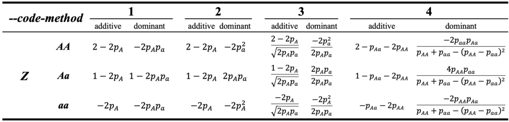
where p_{A} and p_{a} are the allele frequency of A and a, respectively. p_{AA}, p_{Aa} and p_{aa} are the genotype frequency of AA, Aa, aa, respectively.
Users can easily switch to any of method above by specifying the flag --code-method with corresponding value, e.g. --code-method 2. The reference for different methods can be found at the following papers:
--code-method 1, (default) Su, Guosheng, et al. “Estimating additive and non-additive genetic variances and predicting genetic merits using genome-wide dense single nucleotide polymorphism markers.” Plos one (2012): e45293.--code-method 2, Zeng, Zhao-Bang, Tao Wang, and Wei Zou. “Modeling quantitative trait loci and interpretation of models.” Genetics 169.3 (2005): 1711-1725.--code-method 3, Yang, Jian, et al. “Common SNPs explain a large proportion of the heritability for human height.” Nature genetics 42.7 (2010): 565-569.--code-method 4, Vitezica, Zulma G., et al. “Orthogonal estimates of variances for additive, dominance, and epistatic effects in populations.” Genetics 206.3 (2017): 1297-1307.
General GRM
The script to construct additive and dominant genomic relationship matrix:
# construct A and D simultaneously
./hiblup --make-xrm --code-method 2
         --bfile demo
         --add --dom
         --step 10000
         --thread 32
         --out demo
         #--write-txt  #to output a readable ".txt" file
Files named demo.GA.bin, demo.GA.id, demo.GD.bin, demo.GD.id will be generated in the work directory, and HIBLUP will directly compute the inverse of the GRM and output it if --add-inv or --dom-inv is detected in the command.
Note that users can assign a file listing the names of SNPs to the flag --extract or --exclude to construct GRM by a subset of SNPs. For example, constructing GRM only uses the significant SNPs:
./hiblup --make-xrm
         --bfile demo
         --add
         --extract sig.snp.txt
         --thread 32
         --out demo
where the file sig.snp.txt contains the SNPs which are considered to be significantly associated with a trait.
Mixed GRM for multiple populations
HIBLUP can construct a mixed GRM if the genotype data has multiple populations (e.g., different breeds), the mathematical formula of mixed GRM can be expressed as follows:
\begin{equation}
\begin{aligned}
G = \left[\begin{matrix}G_{ii}&G_{ij}\\G_{ji}&G_{jj}\\\end{matrix}\right]=\left[\begin{matrix}\frac{Z_{i}Z_{i}^\top}{tr(Z_{i}Z_{i}^\top)/n_{i}}&\frac{Z_{i}Z_{j}^\top}{\sqrt{tr(Z_{i}Z_{i}^\top)\ast tr(Z_{j}Z_{j}^\top)/(n_{i}\ast n_{j})}}\\\frac{Z_{j}Z_{i}^\top}{\sqrt{tr(Z_{j}Z_{j}^\top)\ast tr(Z_{i}Z_{i}^\top)/(n_{j}\ast n_{i})}}&\frac{Z_{j}Z_{j}^\top}{tr(Z_{j}Z_{j}^\top)/n_{j}}\\\end{matrix}\right]
\end{aligned}
\end{equation}
where Z_{i} and Z_{j} are the centered or scaled genotype matrix (as shown in above Table 1) using corresponding allele frequency or genotype frequency of i_{th} and j_{th} population, respectively. n_{i} and n_{j} are the sample size of different populations.
It’s pretty easy to implement by just providing a population classification file (see file format here) when running HIBLUP to construct a regular GRM:
# construct mixed GRM
./hiblup --make-xrm --code-method 1
         --bfile demo
         --pop-class demo.popclass.txt
         --step 10000
         --thread 32
         --out demo
Weighted GRM
HIBLUP supports to compute the weighted GRM by the following script:
./hiblup --make-xrm --code-method 1
         --bfile demo
         --add --dom
         --snp-weight snp.wt.txt
         --thread 32
         --out demo
The file format of SNP weights please refer to here.
Pedigree and Genome based relationship matrix (HRM)
When pedigree and genome information are provided simultaneously, HIBLUP will automatically construct H matrix following the equation below (Aguilar 2010, Christensen 2010):
\begin{equation}
H =
\begin{bmatrix}
A_{11} + A_{12} A_{22}^{-1} (G_w - A_{22}) A_{22}^{-1} A_{21} & A_{12}A_{22}^{-1}G_w \\
G_wA_{22}^{-1}A_{21} & G_w \\
\end{bmatrix}
\end{equation}
where A_{11} and A_{22} are the submatrices of A matrix for non-genotyped and genotyped individuals, respectively; A_{12} and A_{21} are the submatrices of A matrix, which represent the relationships between genotyped and nongenotyped individuals, G_w = (1 - alpha) * G_{adj} + alpha * A_{22}, G_{adj} is adjusted from the original genomic relastionship matrix G by simple linear regression:
\begin{equation}
\begin{aligned}
Avg(diag(G)) * a + b = Avg(diag(A_{22})) \\
Avg(offdiag(G)) * a + b = Avg(offdiag(A_{22}))
\end{aligned}
\end{equation}
Then we have G_{adj} = G * a + b.
./hiblup --make-xrm
         --pedigree demo.ped
         --bfile demo
         --alpha 0.05
         --add --dom
         --out demo
The above command will generate additive and dominant relationship matrix simultaneously, the filenames are: demo.HA.bin, demo.HA.id, demo.HD.bin, demo.HD.id.
Users can also specify --snp-weight to construct a weighted GRM or specify --pop-class to construct a mixed GRM for constructing HRM.
Besides providing binary genotype to construct HRM, users can also use their own pre-computed GRM to construct HRM, but the pre-computed GRM should be stored in binary format, which can be transformed from square or triangle text file by HIBLUP (see Format conversion of XRM), the corresponding commands are as follows:
./hiblup --make-xrm
         --pedigree demo.ped
         --xrm yourGRM     # yourGRM.bin, yourGRM.id
         --alpha 0.05
         --add             # or '--dom' is supported
         --out demo
Also, HIBLUP can construct the inverse of H matrix by following script:
./hiblup --make-xrm
         --pedigree demo.ped
         --bfile demo
         --alpha 0.05
         --add-inv --dom-inv
         --out demo
the generated filenames are: demo.HAinv.sparse.bin, demo.HAinv.sparse.id, demo.HDinv.sparse.bin, demo.HD.sparse.id.
As described above, you can also construct the inverse of HRM using your own pre-computed GRM.
XRM for environmental random effect
Except for constructing XRM for genetic random effect, HIBLUP can also construct XRM for environmental random effect, phenotype file should be provided for this case, the command is as following:
./hiblup --make-xrm
         --pheno demo.phe
         --rand 6,7
         --out demo
the generated filenames are: demo.loc.sparse.bin, demo.lco.sparse.id, demo.dam.sparse.bin, demo.dam.sparse.id.
NOTE
(1) All above relationship matrix, except for those whose prefix contain character “.sparse.”, can be used by GCTA, LDAK, but additional processes are needed, for example:
awk '{print $1,$1}' demo.GA.id > gcta.grm.id
cp demo.GA.bin gcta.grm.bin
# then use it by GCTA
./gcta64 ... --grm gcta ...
(2) The binary format relationship matrix calculated by GCTA or LDAK can be used directly by HIBLUP without any format transformation, just assign its prefix to flag --xrm.
3.7.Format conversion of XRM
HIBLUP only accept XRM in binary file format, as some software (e.g. DMU, BLUPF90, ASReml) can not recognize it, moreover, it would be hard for programming beginners to prepare those binary files, we therefore provide a format converter for easily linking HIBLUP with other software.
Binary to text
The following command will output the XRM into a square matrix in text format with names of demo.txt and demo.id.txt:
./hiblup --trans-xrm
         --xrm demo.GA
         --out demo
#        --triangle
An example for demo.txt with three individuals is as follows:
1.55755	1.04847	0.64622
1.04847	1.58144	0.66971
0.64622	0.66971	1.56794
If the flag --triangle is detected, HIBLUP will only write the lower triangle of the matrix into text file with format of <i j k>, where i, j, k are the row, column index, and its corresponding value respectively. For sparse matrix, HIBLUP will ignore zero elements when outputting “ijk” format. An example file with the same three individuals above is shown below:
1	1	1.55755
2	1	1.04847
2	2	1.58144
3	1	0.646224
3	2	0.669715
3	3	1.56794
Text to binary
If users have their own prior calculated relationship matrix in text format, HIBLUP can transform it into binary file, which can be used by HIBLUP directly, the script is as following:
./hiblup --trans-xrm
         --xrm-txt demo.txt
         --xrm-id demo.id.txt
         --out demo
Above command requires demo.txt in square format and demo.id.txt. If the file demo.txt is in “ijk” format, please remember to add flag --triangle.
NOTE
HIBLUP can also convert the relationship matrix calculated by GCTA, LDAK to text format:
./hiblup --trans-xrm --xrm gcta.grm --out hiblup
3.8.Calculate inbreeding and relationship coefficient
Inbreeding and relationship coefficients are derived from either pedigree or genotype information, HIBLUP firstly constructs additive numerator matrix, then derive and output the coefficients in file. The flag for inbreeding coefficient and relationship coefficient is --ibc and --rc, respectively.
Inbreeding coefficients
# derived from pedigree
./hiblup --ibc --pedigree demo.ped --thread 32 --out demo
# or derived from prior calculated PA matrix
./hiblup --ibc --xrm demo.PA --out demo

# derived from genotype
./hiblup --ibc --bfile demo --thread 32 --out demo
# or derived from prior calculated GA matrix
./hiblup --ibc --xrm demo.GA --out demo
The inbreeding coefficients are saved in file demo.ibc:
id        ibc
IND0702  0.00290048
IND0703  0.00262272
IND0704  0.00262272
Relationship coefficients
# derived from pedigree
./hiblup --rc --pedigree demo.ped --thread 32 --out demo
# or derived from prior calculated PA matrix
./hiblup --rc --xrm demo.PA --out demo

# derived from genotype
./hiblup --rc --bfile demo --thread 32 --out demo
# or derived from prior calculated GA matrix
./hiblup --rc --xrm demo.GA --out demo
The relationship coefficients are saved in file demo.rc:
id1     id2     rc
IND0701 IND0701 1
IND0701 IND0702 0.472652
IND0701 IND0703 0.0721178
IND0701 IND0704 0.0721178
NOTE
1. The inbreeding coefficients and relationship coefficients can be calculated at a time, like:
./hiblup --ibc --rc --pedigree demo.ped --out demo
./hiblup --ibc --rc --bfile demo --out demo
2. The genomic inbreeding coefficients and relationship coefficients can be calculated by different methods using the flag --code-method, more details can be seen here.
./hiblup --ibc --rc --bfile demo --code-method 1 --out demo
3.9.Principal component analysis
HIBLUP has the function of calculating PCA for a population, the genotype or the relationship matrix should be provided.
Calculating PCs from genotype
./hiblup --pca --bfile demo --out demo
Note that user can add flag --step n to control the memory cost, and specify flag --npc n to output several number of PCs instead of all.
Calculating PCs from XRM
./hiblup --pca --xrm demo.GA --npc 5 --out demo
There are two files demo.pc and demo.pcp will be generated.
The file demo.pc contains the calculated PCs, overview of the file:
id       PC1     PC2     PC3     PC4     PC5
IND0701  0.0413326       -0.00664808     -0.00795809     0.0218009       -0.0156735
IND0702  0.00856316      0.0378125       0.000503819     0.0205049       0.00972465
IND0703  -0.00793242     0.0458023       -0.00438572     -0.0173733      -0.0254701
IND0704  -0.00793248     0.0458023       -0.00438575     -0.0173733      -0.0254701
The file demo.pcp contains the Proportion and Cumulative Proportion of variance of PCs, overview of the file:
Components      PC1     PC2     PC3     PC4     PC5
Standard deviation      4.23976    4.10211    3.76024    3.66821    3.60725
Proportion of Variance  0.0224695  0.0210342  0.0176743  0.0168197  0.0162653
Cumulative Proportion   0.0224695  0.0435037  0.0611779  0.0779976  0.094263
3.10.LM, BLUP, PBLUP, GBLUP(rrBLUP), SSGBLUP
Users can easily implement simple linear model (LM), BLUP, PBLUP, GBLUP (rrBLUP) and SSGBLUP, HIBLUP can automatically switch to one of them according to the data type provided by users. The following table details the required or non-required flags for different model in HIBLUP:
| Model | –qcovar/–dcovcar | –rand | –pedigree | –bfile |
|---|---|---|---|---|
| LM | √ | × | × | × |
| BLUP | O | √ | O | O |
| PBLUP | O | O | √ | × |
| GBLUP | O | O | × | √ |
| SSGBLUP | O | O | √ | √ |
√: required; ×: not required; O: optional.
rrBLUP model is theoretically the same with GBLUP model, users can just add a flag --snp-effect on the base of GBLUP model to obtain the SNP effect for rrBLUP model.
IMPORTANT
It should be noted that, the PBLUP model can be pretty efficient owing to the high performance of FSPAK technology on the very sparse ‘LHS’ of mixed model equation. However, HIBLUP is designed for genome-based genetic evaluation, in which the ‘LHS’ is no longer sparse, the ‘V’ matrix based strategy that is achieved in HIBLUP would be more competent for this case. Although users can fit PBLUP model by using HIBLUP, it may be slower and memory-costing compared with those of the software, e.g., DMU, BLUPF90. Therefore, we recommend using DMU or BLUPF90 when fitting a model only involves pedigree information.
3.11.Single trait model
Single trait model aims to estimate variance components and its heritability of all random effects for a trait. Always remember that there is no need to adjust the order of individuals or markers to be consistent among different files, HIBLUP can do it automatically. Example command of running SSGLBUP for single trait model:
./hiblup --single-trait
         --pheno demo.phe
         --pheno-pos 8
         --dcovar 2,3       #fixed effect
         --qcovar 4,5       #covariates
         --rand 6,7         #non-genetic (environmental) random effect
         --pedigree demo.ped    #genetic random effect
         --bfile demo           #genetic random effect
         --add --dom
         --threads 32
         --out demo
The detailed format of input files please refer to phenotype, genotype. The way of how to set covariates (--qcovar), fixed (--dcovar) and random (--rand) effect for multiple traits, please refer to here.
Note that all the parameters (e.g., weighted GRM, mixed GRM, or HRM, …) supported for XRM construction can also be applied in the above command.
There are 5 types of algorithms for variance components estimation:
“AI”, “EM”, “HE”, “EMAI”, “HI”, where “AI” is AIREML,”EM” is EMREML, and “HE” represents HE regression, “HI” is “HE+AI”, which uses the outcome of HE regression as the start values of AIREML, users can choose one of them by flag --vc-method, and change the maximum iteration number for AIREML and EMREML by flag --ai-maxit and --em-maxit respectively. For “HE” regression, if covariates for fixed effects are provided, HIBLUP will first regress the phenotype on these, then perform HE Regression using the residuals, the standard error(SE) of HE is computed by Jackknife resampling strategy at 100 repeats. By default, HIBLUP doesn’t calculate the random effects for HE regression, user can add a flag --he-pred to output it, and only in this situation, the flag --pcg can be used for fast computing on very large dataset, which we call it as “HE+PCG” strategy.
However, above command maybe time-consuming when fitting trait by trait, as it repeatedly constructs XRM for each trait. We can construct XRM only once at the beginning, then assign it to --xrm when fitting multiple traits, which can give the same results, but would be much more efficient, the command can be referred as following:
# Step 1: construct XRMs
./hiblup --make-xrm
         --pedigree demo.ped
         --bfile demo
         --add --dom
         --out demo

# Step 2: link XRMs to fit model
./hiblup --single-trait
         --pheno demo.phe
         --pheno-pos 8
         --dcovar 2,3
         --qcovar 4,5
         --rand 6,7
         --xrm demo.HA,demo.HD
         --add --dom
         --threads 32
         --out demo
Several files will be generated in the work directory:demo.vars: the estimated variance and heritability of all random effects:
	Var	Var_SE	h2	h2_SE
loc	12.2127	8.9109	0.1035	0.0682
dam	10.6268	4.8605	0.0901	0.041
HA	59.2007	11.7641	0.5019	0.0807
HD	28.9946	8.9294	0.2458	0.083
e	6.9232	1.6957	0.0587	0.0161
demo.beta: the estimated coefficients of all covariates and fixed effects:
Levels	Estimation	SE
mu	32.5285	3.4758
sex_F	6.2933	1.7593
sex_M	26.2353	1.7634
season_Autumn	18.0905	0.9753
season_Spring	-1.9168	0.9904
season_Summer	7.8471	1.0066
season_Winter	8.5078	0.9944
day	0.1547	0.0574
bornweight	1.5703	0.4614
demo.anova: analysis of variance table of all covariates and fixed effects:
Factors	Df	SumSq	MeanSq	F	Pr(>F)
sex	1	49710.3845	49710.3845	7180.311	<2e-16
season	3	24515.0941	8171.698	1180.344	<2e-16
day	1	925.3352	925.3352	133.658	<2e-16
bornweight	1	437.3432	437.3432	63.171	1.30E-14
e	493	3413.1141	6.9232
demo.rand: the estimated environmental random effects, genetic random effects (the column named “PA”, “GA”, or “HA” is the list of breeding values for phenotypic and non-phenotypic individuals) and residuals.
Users can specify the start values for all unknown variance to --vc-priors for fast convergence, the way of how to input the variance components can be found at here.
3.12.Repeat records of single trait model
Running repeat records model is nearly the same with fitting single trait model, the only difference is that repeat records model can fit the permanent environment effect, which can be achieved by assigning individual id at the first column of phenotype file to environmental random effect, take GBLUP model for an example:
./hiblup --single-trait
         --pheno demo.repeat.phe
         --pheno-pos 2
         --rand 1
         --bfile demo
         --threads 32
         --out demo
It should be noted that HIBLUP uses the variance-covariance matrix of phenotype records in genetic parameter estimation, thus if there are low-replications (e.g., 2000 records from 1000 individuals replicated twice), HIBLUP will be faster than MME-based software. But if the analyzed trait are highly replicated (e.g., 2000 records from 200 individuals replicated 10 times), the BLUPF90, ASreml or other MME-based algorithms will be much faster and we recommend you to use that software.
3.13.Multiple traits model
Multiple traits model is used for estimating genetic correlation among traits of one population or the same traits of multiple populations, both balanced or unbalanced records (v 1.5.0 or later) are now acceptable and there is no limitation on the number of traits used in analysis for HIBLUP. Moreover, users can appoint different covariates, fixed and random effects for different traits. PBLUP, GBLUP, SSGBLUP are all available for multiple traits model, HIBLUP can automatically switch to one of them according to the provided file. Always remember that there is no need to adjust the order of individuals or markers to be consistent among different files, HIBLUP can do it automatically.
Taking GBLUP for an example, the multiple model can be achieved by following command:
./hiblup --multi-trait
         --pheno demo.phe
         --pheno-pos 8 9 10
         --qcovar 4,5 5 4
         --dcovar 2,3 0 2
         --rand 6,7 7 0
         --xrm demo.GA,demo.GD  # same with --bfile demo --add --dom
         --vc-method AI
         --ai-maxit 30
         --threads 32
         --out demo
The detailed format of input files please refer to phenotype, genotype. The way of how to set covariates (--qcovar), fixed (--dcovar) and random (--rand) effect for multiple traits, please refer to here.
There are 5 types of algorithms for variance components estimation:
“AI”, “EM”, “HE”, “EMAI”, “HI”, where “AI” is AIREML,”EM” is EMREML, and “HE” represents HE regression, “HI” is “HE+AI”, which uses the outcome of HE regression as the start values of AIREML, users can choose one of them by flag --vc-method, and change the maximum iteration number for AIREML and EMREML by flag --ai-maxit and --em-maxit respectively. For “HE” regression, if covariates for fixed effects are provided, HIBLUP will first regress the phenotype on these, then perform HE Regression using the residuals, the standard error(SE) of HE is computed by Jackknife resampling strategy at 100 repeats. By default, HIBLUP doesn’t calculate the random effects for HE regression, user can add a flag --he-pred to output it, and only in this situation, the flag --pcg can be used for fast computing on very large dataset, which we call it as “HE+PCG” strategy.
By default, HIBLUP fits the covariance of residuals among traits, users can add the flag --ignore-cove to ignore residual covariance for multiple traits model.
Several files will be generated:
demo.vars: the variance, heritability and SE of all random effects for all traits:
Item	Var	Var_SE	h2	h2_SE
tr1_loc	13.73854	9.9309	0.11739	0.07538
tr1_dam	2.29288	3.18932	0.01959	0.02731
tr1_demo.GA	61.35173	9.57171	0.52423	0.06964
tr1_demo.GD	29.93077	6.27996	0.25575	0.06022
tr1_e	9.71917	1.67088	0.08305	0.01696
tr2_dam	3.42172	3.80424	0.02971	0.03308
tr2_demo.GA	63.59	10.52058	0.55219	0.06017
tr2_demo.GD	38.14332	7.27491	0.33122	0.06696
tr2_e	10.00395	1.63578	0.08687	0.01578
tr3_demo.GA	21.03906	6.94184	0.2203	0.0668
tr3_demo.GD	15.25593	10.56861	0.15974	0.10919
tr3_e	59.20689	9.04084	0.61996	0.09801
demo.covars: the co-variance, correlation and SE of all traits for all genetic random effects:
Item	COVar	COVar_SE	r	r_SE
tr1:tr2_demo.GA	46.6899	8.56852	0.747524	0.171364
tr1:tr3_demo.GA	16.3376	5.96333	0.454749	0.185599
tr2:tr3_demo.GA	12.3489	6.21401	0.337612	0.157671
tr1:tr2_demo.GD	26.9273	4.65452	0.796922	0
tr1:tr3_demo.GD	-2.25039	4.95673	-0.105301	0.23413
tr2:tr3_demo.GD	8.23124	5.21494	0.341194	0.259133
tr1:tr2_e	0.24039	1.17428	0.024379	0.119333
tr1:tr3_e	-1.10713	2.87487	-0.0461537	0.11985
tr2:tr3_e	-4.80127	2.85341	-0.197284	0.128375
demo.*.anova: the variance analysis table of covariates, fixed effects for different traits.demo.*.beta: the estimated coefficients and SE of covariates, fixed effects for different traits.demo.*.rand: the estimated environmental random effects, genetic random effects (the column named “PA”, “GA”, or “HA” is the list of breeding values for phenotypic and non-phenotypic individuals) and residuals for different traits.
Users can specify the start values for all unknown variance and co-variance to --vc-priors and --covc-priors, the way of how to input the genetic components can be found at here.
NOTE
HIBLUP only estimates co-variance for genetic random effect and residual effect, not for environmental random effect, therefore at least one genetic random effect should be included in the model, which can be from pedigree (--pedigree), genotype (--bfile) or XRMs (--xrm). If users insist on estimating correlation for environmental random effects, just make relationship matrix for those random effects by the flag --make-xrm (see the chapter “XRM for environmental random effect” here), then assign it to the option --xrm.
3.14.Solve mixed model equation
The objective of solving mixed model is to obtain the estimated breeding values of all individuals by using the known genetic parameters. HIBLUP automatically switches to single trait or multiple traits model by the length of specified flag --pheno-pos. Always remember that there is no need to adjust the order of individuals or markers to be consistent among different files, HIBLUP can do it automatically.
Taking GBLUP model for an example, the command for single trait and multiple traits model is as following:
# (1) additive effect for single trait model
./hiblup --mme
         --pheno demo.phe
         --pheno-pos 8
         --rand 6
         --xrm demo.GA   # can be replaced by --bfile demo --add
         --vc-priors v1,v2,v3
         --pcg
         --threads 32
         --out demo

# (2) additive and dominant effect for multiple traits model
./hiblup --mme
         --pheno demo.phe
         --pheno-pos 8 9 10
         --rand 6,7 7 0
         --bfile demo   # can be replaced by --xrm demo.GA,demo.GD
         --add --dom
         --vc-priors t1_v1,t1_v2,t1_v3,t1_v4,t1_v5 t2_v1,
                     t2_v2,t2_v3,t2_v4 t3_v1,t3_v2,t3_v3
         --covc-priors cov1,cov2,cov3 cov4,cov5,cov6 cov7,cov8,cov9
         --pcg
         --threads 32
         --out demo
By default, HIBLUP directly compute the inverse of V matrix, users can try to add flag --pcg to use Preconditioned Conjugate Gradients algorithm to solve the system of linear equation, which is much more faster in certain situation.
IMPORTANT
(1) --vc-priors contains the variance components of all random effects, including environmental random effects, genetic random effects, and residuals, the provided variance components should also be in this order.
For single trait model, please use comma as separator, as shown in the first example command:
v1: the variance of the environmental random effect located
    at the 6th column in phenotype file.
v2: the additive genetic variance.
v3: the residual variance.
For multiple traits model, the variance components are listed trait by trait orderly, and please use comma within a trait, use space among traits, as shown in the second example command:
t1_v1: the variance of the environmental random effect located
       at the 6th column in phenotype file for the first trait.
t1_v2: the variance of the environmental random effect located
       at the 7th column in phenotype file for the first trait.
t1_v3: the variance of additive genetic effect for the first trait.
t1_v4: the variance of dominant genetic effect for the first trait.
t1_v5: the variance of residuals for the first trait.
t2_v1: the variance of the environmental random effect located
       at the 7th column in phenotype file for the second trait.
t2_v2: the variance of additive genetic effect for the second trait.
t2_v3: the variance of dominant genetic effect for the second trait.
t2_v4: the variance of residuals for the second trait.
t3_v1: the variance of additive genetic effect for the third trait.
t3_v2: the variance of dominant genetic effect for the third trait.
t3_v3: the variance of residuals for the third trait.
(2) --covc-priors contains the co-variance components among traits at all genetic random effects, the co-variance components are listed by genetic random effect orderly, and please use comma within a genetic random effect, use space among genetic random effects, the input order can be referred as following:

where each box represents a genetic random effect, the off-diagonals are the co-variances between traits at this genetic random effect, and the diagonals are its variance at different traits. The number of box is equal to the number of XRM plus 1, where “1” is the residual. Users need to assign values at the lower triangle of each box to HIBLUP:
cov1: the co-variance between the first and second trait at "demo.GA".
cov2: the co-variance between the first and third trait at "demo.GA".
cov3: the co-variance between the second and third trait at "demo.GA".
...
The order of input co-variances should strictly follow the route in the above figure.
3.15.Fitting interaction for effects
Environmental interaction (E by E)
Interaction between recorded environments can be fitted as fixed or random effects, please use colon as separator.
If fitted as fixed effects:
./hiblup ... --dcovar 2,2:3:6
Above command represents that the fixed effects of this trait are “sex“, the interaction among “sex“, “season“, “loc“.
If fitted as random effects:
./hiblup ... --rand 6,6:7,7
Similarly, the random effect for this trait are “loc“, the interaction between “loc” and “dam“, and “dam“.
For multiple trait model, use space for separator, take 3 traits for an example:
./hiblup ... --dcovar 2:3 0 2,3,2:3 --rand 6 7,6:7 0
which means the fixed effect for the first trait is the interaction between “sex“, “season“, no fixed effect for the second trait, the fixed effects of the third trait are “sex“, “season“, and the interaction between “sex“, “season“; the environmental random effects for the first trait is “loc“, the second trait are “dam“and the interaction between “loc” and “dam“, the third trait has no environmental random effect.
Genetic interaction (G by G)
HIBLUP can fit interaction for genetic random effect, for example: additive by additive, additive (A) by dominant (D), dominant by dominant, and so on, the number of genetic random effect at an interaction term is not limited. The interaction of G by G for n genetic random effects in HIBLUP can be mathematically formulated as following:
\begin{equation}
\begin{aligned}
G_{inter} &= \frac{G_1 \bigodot G_2 \bigodot ... \bigodot G_n}{tr(G_1 \bigodot G_2 \bigodot ... \bigodot G_n) / N}
\end{aligned}
\end{equation}
where N is the number of individuals, \bigodot is the Hadamard product (i.e. element-wise multiplica-tion) of all matrix, and tr() is the trace of the matrix.
The only way to fit G by G is to appoint the prefix of the random effects to flag --xrm, please use colon as separator within an interaction term:
# fit A by D only
./hiblup ... --xrm demo.GA:demo.GD
#fit A, D, and A by D
./hiblup ... --xrm demo.GA,demo.GD,demo.GA:demo.GD
#fit A by A, A by D and D by D simultaneously
./hiblup ... --xrm demo.GA:demo.GA,demo.GA:demo.GD,demo.GD:demo.GD
Genetic-Environmental interaction (G by E)
Genetic-Environmental interaction will be included in the model as random effect, please assign a digital value representing its position at phenotype file for environment factors, and assign prefix of the genetic effects to the flag “--rand-gxe“.
For single trait model, please use colon as separator within an interaction term, and use comma as separator for multiple interaction terms, for example:
./hiblup --single-trait ... --rand-gxe 6:demo.GA,6:demo.GD
#interaction among multiple effects
./hiblup --single-trait ... --rand-gxe 6:demo.GA:demo.GD
./hiblup --single-trait ... --rand-gxe 6:7:demo.GA
For multiple traits model, please use space among traits, use 0 if there is no G by E interaction to be considered for a trait, take 3 traits for an example:
./hiblup --multi-traits ... --rand-gxe 6:demo.GA 6:demo.GA,7:demo.GA 0
Above command means that the interaction for the first trait is “loc” by additive genetic effect; the interactions for the second trait are “loc” by additive genetic effect and “dam” by additive genetic effect; no interactions are considered for the third trait.
3.16.Statistical tests of significance for effects
For fixed effects and covariates, HIBLUP can do statistical test automatically, and list the results in file *.anova, the p-value of F test at the last column could be used as a diagnosis of which fixed effects or covariates are statistically significant for a trait.
For random effect (genetic or environmental), there is no automatic function of statistical test for significance, users can achieve it manually by the Likelihood Ratio Test (LRT) following the steps below:
(1) run full model with the random effect of interest, get the loglike value L1 (which can be found from the LOG information of HIBLUP at the last iteration of REML).
(2) run reduced model in which the random effect of interest is dropped off, get the loglike value L0.
(3) calculate the p-value by Chi-square test in R:
> stat <- 2 * (L1 - L0)
> pvaue <- pchisq(stat, df = 1, lower.tail = FALSE)
> print(pvaue)
3.17.Reliability and PEV
For single trait model, multiple traits model and solving mixed model equation, HIBLUP can calculate the reliability and prediction error variance (PEV) of all random effects. The mathematical formula for reliability calculation is as follows:
\begin{equation}
\begin{aligned}
r^{2} &= 1-\frac{PEV}{\sigma^{2}}
\end{aligned}
\end{equation}
where \sigma^{2} is the estimated variance from REML analysis for the random effect of interest. The prediction error variance PEV can be obtained from the following equation:
\begin{equation}
\begin{aligned}
PEV &= C_{ii}*\sigma_{e}^{2}
\end{aligned}
\end{equation}
where \sigma_e^{2} is the estimated residual variance. C_{ii} is the i_{th} diagonal element of the inverse matrix of left hand side (LHS) of mixed model equation.
By default, HIBLUP does not calculate and output those statistics, as the reliability estimation usually takes longer than whole REML process, thus please add flag --r2 only if you really want to get the reliability.
Taking single trait model for an example, the script to obtain the reliability is as follows:
./hiblup --single-trait
         --pheno demo.phe
         --pheno-pos 8
         --dcovar 2,3       #fixed effect
         --qcovar 4,5       #covariates
         --rand 7           #non-genetic (environmental) random effect
         --bfile demo       #genetic random effect
         --r2               #to calculate the reliability
         --threads 32
         --out demo
Then each random effect, including residual, has several additional columns listing its corresponding standard error, PEV and reliability, overview of the file:
ID      dam       dam_SE   dam_PEV  dam_R2    GA        GA_SE    GA_PEV   GA_R2     residuals  residuals_SE residuals_PEV residuals_R2
IND1001 0.496645  3.75992  14.137   0.255863  6.66127   4.27597  18.2839  0.774767  -1.45194   3.18313      10.1323       0.55248
IND1002 0.496645  3.75992  14.137   0.255863  6.66127   4.27597  18.2839  0.774767  2.04383    3.17906      10.1064       0.553624
IND1003 0.674833  3.53678  12.5088  0.341566  2.08201   4.62091  21.3528  0.736963  -0.104053  4.14567      17.1866       0.24091
IND1004 0.674833  3.53678  12.5088  0.341566  -0.682836 4.70199  22.1087  0.727651  0.9083     4.17824      17.4577       0.228936
3.18.Compute SNP effect
HIBLUP now can compute the additive and dominant effects for all SNPs. There are two ways to compute SNP effects, the first way is to add flag --snp-effect in the command when fitting single trait, multiple traits model, or solving mixed model:
# compute additive SNP effect by SSGBLUP of single trait model
./hiblup --single-trait
         --pheno demo.phe
         --pheno-pos 8
         --bfile demo
         --pedigree demo.ped
         --add
         --snp-effect
         --thread 32
         --out demo
the second way is to derive SNP effect from prior calculated GEBVs:
# compute dominant SNP effect
./hiblup --snp-effect
         --gebv demo.gebv.d.txt
         --bfile demo
         --dom
         --thread 32
         --out demo
The file format of GEBVs can be found at here. The genotype file specified by --bfile is used to construct GRM and compute SNP effect, for the second way, HIBLUP will construct additive or dominant GRM for individuals, to save time, users can provide prior calculated GRM, HIBLUP will use it directly:
# compute additive and dominant SNP effect
./hiblup --snp-effect
         --gebv demo.gebv.ad.txt
         --bfile demo
         --xrm demo.GA,demo.GD
         --add --dom
         --thread 32
         --out demo
The SNP effects of all SNPs are stored in file demo.snpeff.
NOTE
If the GEBVs are calculated by using a weight GRM, please remember to provide the same weights of all SNPs to flag --snp-weight.
3.19.Predicting GEBV/GPRS
HIBLUP has the function of predicting genomic estimated breeding value (GEBV) or genomic polygenic risk score (GPRS) using the pre-computed SNP effects and individual level genotype data, which is the same with the function “--score” in PLINK software, but several times faster for computing.
The command to do prediction is as follows:
./hiblup --pred
         --bfile demo        #the binary genotype data
         --score demo.snpeff #the pre-computed SNP effects
         --threads 10
         --out demo
Note that the genotype should be in PLINK binary file, and at least 5 columns should be included in SNP effects file (see detailed format here). By default, HIBLUP codes the genotype in additive genetic effect (i.e., 0 1 2 for AA Aa aa), user can add a flag “--dom” to code the genotype in dominant effect (i.e., 0 1 0 for AA Aa aa) if the provided SNPs effects are all in dominant. But if both “--add” and “--dom” are specified in commands, the SNP effect file must have 6 columns, of which the 5th and 6th are the additive and dominant SNP effects, respectively. Thus, if there are additive and dominant effects in file, please remember to add flag “--add --dom” in the commands.
A file named “demo.bv” will be generated in the work directory, overview of this file:
id	trait1	trait2
Ind2	-0.305403	2.6644
Ind5	0.00897198	-1.36166
Ind11	0.392148	-0.653216
Ind17	0.00232218	-0.213599
Ind22	-0.359507	-2.12692
Ind45	-0.232806	0.269005
As shown above, the first column is the individual id, and the rest of columns are the predicted GEBV or GPRS, the number of columns depends on the number of effects provided in SNP effects file.
3.20.Genomic mating
Genomic mating is a technology unionizing all available SNPs to predict the expected genetic performance of progeny for all combinations between males and females (Tang, et al. 2023). To implement genomic mating, genotype of all individuals and additive or dominant effects of all SNPs should be provided. The format of SNP effect file can be found at here. The command to do genomic mating by HIBLUP is as following:
./hiblup --mating
         --bfile demo
         --score demo.snpeff
         --thread 32
         --out demo
Mating results are saved in file demo.mating, brief view of this file:
sir 	 dam 	 g
Ind704 	 Ind710 	 -0.0675817
Ind704 	 Ind711 	 1.06056
Ind704 	 Ind712 	 2.00997
Ind704 	 Ind713 	 -0.0879987
Ind704 	 Ind714 	-0.492576
The last column is the expected genetic performance of progeny for different combinations.
IMPORTANT
(1) The SNP with the same name between demo.bim and demo.snpeff should have the consistent reference (A1) and alternative (A2) allele.
(2) All the individuals in demo.fam should be clearly marked with gender (located at the 5th column, 1=male; 2=female; other=unknown), any individual with unknown gender will be deleted in analysis.
3.21.LD
HIBLUP has the function of calculating LD correlation (r) for pairwise SNPs based on genotype allele counts. The commands are as follows:
./hiblup --ld
         --bfile demo
         --window-bp 1e6
         --threads 16
         --out demo_ldm
Two files (*.info, *.bin) will be generated in the folder. Since the binary file (*.bin) cannot be opened directly, users can add a flag --write-txt in the above commands to output a readable “.txt” file.
There are several options to set the window size:
--window-bp: to specify the size of non-overlapped window (default 1Mb, i.e.,--window-bp 1000000), in which the number of SNPs is not fixed;--window-num: to specify a fixed number of SNPs in a window (e.g.,--window-num 500), the size of window is not constant in this case;--window-geno: to define all SNPs across entire genome as one window, note that it will take a long time and huge memory cost if there are large number of SNPs;--window-file: to specify a text file in which the windows are pre-defined by users, see the file format here.
3.22.LD scores
The LD score is defined as the sum of LD (r2 ) between a SNP and all the SNPs in a region, it reflects the linkage level of a SNP with other SNPs, higher LD score represents that this SNP is higher correlated with others. The LD scores are generally used in LD score regression to estimate the heritability of a trait or the genetic correlation between traits. To obtain the LD scores of SNPs, the individual level genotype data is required, see the following example:
./hiblup --ldscore
         --bfile demo
         --window-bp 1000000
         --threads 10
         --out test
There are several options to set the window size:
--window-bp: to specify the size of non-overlapped window (default 1Mb, i.e.,--window-bp 1000000), in which the number of SNPs is not fixed;--window-num: to specify a fixed number of SNPs in a window (e.g.,--window-num 500), the size of window is not constant in this case;--window-geno: to define all SNPs across entire genome as one window, note that it will take a long time and huge memory cost if there are large number of SNPs;--window-file: to specify a text file in which the windows are pre-defined by users, see the file format here.
A file named “test.ldsc” will be generated in the work directory, overview of this file:
id	maf	ldscore
M1	0.481875	1
M2	0.145	1
M3	0.320625	1
.	.	.
.	.	.
.	.	.
M991	0.089375	1.044
M992	0.11375	1.33231
M993	0.31875	1.2885
M994	0.103125	1
M995	0.115625	1
As shown above, the first column is the vector of SNP names, the second is minor allele frequency, the third is the calculated LD scores.
Users can also use the publicly available LD scores file to run HIBLUP, but sometimes the column “maf” is missing. Since HIBLUP uses the “maf” column to set the options “--M” by counting the number of markers with MAF >= 0.05, thus if the option “--M” is specified when running LD score regression (e.g., the value in the file “XXX.M_5_50“), the “maf” column will be useless, users can assign any dummy values to this column.
3.23.LD score regression
LD score regression is method widely used in summary statistics to estimate the heritability of a trait (Bulik-Sullivan, Po-Ru Loh, et al. 2015) and the genetic correlation among traits (Bulik-Sullivan, Finucane, et al. 2015). It doesn’t require individual level genotype data, only the GWAS summary data and the LD scores calculated from reference panel are involved, thus it’s pretty time-efficient and memory-saving compared with REML or HE regression.
1. Heritability estimation
./hiblup --ldreg
         --sumstat demo.ma   #the summary data
         --lds demo.ldsc     #the pre-computed LD scores
         --out demo
As shown above, the summary data file and LD scores file should be provided, the file format of summary data and how to calculate/make LD scores can be found at other tutorial chapters (i.e., summary data and LD scores). Please always remember not to delete SNPs in LD scores file to keep it consistent with that in summary data file, just leave it as it is, because the total number of SNPs used to calculate this LD scores is quite crucial for LD score regression.
The estimated results are stored in a file named “demo.ldsr.h2“, overview of this file:
Item	Intercept	Intercept_SE	h2	h2_SE	h2_Pval
demo	1.08285	0.011433	0.122826	0.00393122	2.71554e-214
The ‘Intercept‘ is associated with the population structure, the closer it is to 1, the less stratified of the population is. The ‘h2‘ is the estimated heritability of the trait, and ‘h2_Pval‘ is the p-value of chi-square testing significance.
2. Genetic correlation estimation
The usage of genetic correlation estimation is quite similar with heritability estimation, if HIBLUP detected more than one summary data file in the command, it will estimate heritability and genetic correlation automatically:
./hiblup --ldreg
         --sumstat demo1.ma demo2.ma demo3.ma   #the summary data of multiple traits, use space as separator
         --lds demo.ldsc     #the pre-computed LD scores
         --out demo
Note that the number of summary data of traits is not limited. Two files will be generated in the work directory: the file “test.ldsr.h2” recorded the estimated heritability of trait as described before; and the file “test.ldsr.rg” stores the genetic correlation of pairs of traits, overview of this file:
Item	CovG	CovG_SE	Intercept	Intercept_SE	rG	rG_SE	rG_Pval
demo1:demo2	0.0252414	0.00716841	0.0166108	0.00819384	0.141956	0.0403148	0.000429607
demo1:demo3	0.0744506	0.00892225	0.102821	0.00671784	0.296832	0.0355727	7.15917e-17
demo2:demo3	0.262124	0.0340515	0.315166	0.0112682	0.608769	0.0790827	1.38348e-14
The ‘CovG‘ is the genetic covariance, ‘rG‘ is the estimated genetic correlation between traits, and ‘rG_Pval‘ is the p-value of chi-square testing significance.
The relevant options can be specified by users for LD score regression:
--M: to specify the number of SNPs in LD score regression. By default, HIBLUP use the number of SNPs in the LD score file with MAF between 5% and 50% as it is suggested by Bulik-Sullivan.--chisq-max: to specify the maximum threshold of X2 for the first step estimator of intercept, the default is 30.--intercept-h2: to constrain the intercept with a constant rather than estimating it from data for heritability estimation.--intercept-gencov: to constrain the intercept with a constant rather than estimating it from data for genetic correlation estimation.
3.24.Summary level BLUP (SBLUP)
SBLUP model is a method to estimate marker effects using summary data from a GWAS/meta-analysis and LD matrix derived from a reference panel with individual-level data (Robinson, et al. 2017). The summary data should be prepared in COJO format, as described here. There are two ways to run SBLUP model by HIBLUP, see details as follows:
1. Run SBLUP using genotype data
The first way to run SBLUP model is to use the genotype data provided directly:
./hiblup --sblup
         --sumstat demo.ma   #the summary data
         --bfile demo
         --window-bp 1e6
         --h2 0.3234
         --threads 16
         --out demo
The command --h2 is the heritability of the trait in analysis, which can be estimated from REML if the individual-level data are available or from LD score regression using the summary data.
There are several options to set the window size:
--window-bp: to specify the size of non-overlapped window (default 1Mb, i.e.,--window-bp 1000000), in which the number of SNPs is not fixed;--window-num: to specify a fixed number of SNPs in a window (e.g.,--window-num 500), the size of window is not constant in this case;--window-geno: to define all SNPs across entire genome as one window, note that it will take a long time and huge memory cost if there are large number of SNPs;--window-file: to specify a text file in which the windows are pre-defined by users, see the file format here.
If the number of SNPs in a defined window size is pretty large (e.g., over 10k), it is recommended to add flag --pcg for fast computing of SNP effects in analysis.
2. Run SBLUP using pre-computed LD correlation matrix
Instead of using genotype data, using the LD correlation matrix to fit SBLUP model is more straight-forward. Although this strategy is more computationally efficient and memory-saving than the first one, it should be noted that all the SNPs should satisfy the Hardy-Weinberg equilibrium. If not, the estimated SNP effects would be biased, resulting in a bad prediction performance.
./hiblup --sblup
         --sumstat demo.ma   #the summary data
         --ldm demo_ldm      #the pre-computed LD correlation matrix
         --h2 0.3234
         --threads 10
         --out demo
The command --ldm is used to specify the LD correlation matrix, which could be computed by HIBLUP using the individual-level genotype data, see more details here. Also, If the number of SNPs in a window is pretty large (e.g., over 10k), it is recommended to add flag --pcg for fast computing of SNP effects in analysis.
After running successfully, a file named “demo.snpeff” will be generated in the work directory as follows:
id a1 a2 freq_a1 demo
M1 A G 0.1285 -0.000963937
M2 T C 0.1285 -0.00108931
M3 A G 0.1062 0.00588629
M4 G A 0.1285 -0.00164344
M5 A C 0.2459 -0.00100206
As shown above, the estimated SNP effects are listed in the last column. To obtain the predicted GEBV or GPRS of individuals, we recommend using HIBLUP to implement it (see here), since we tested that it is several times faster than the ‘--score‘ function in PLINK.
3.25.Multiple traits SBLUP (MT-SBLUP)
The multi-trait SBLUP is extended from single trait SBLUP model, it outperforms single trait SBLUP model on prediction accuracy for all the traits in analysis (Robert, Zhihong, et al. 2018). There are two ways to fit MT-SBLUP model, by either individual genotype data or LD correlation matrix, see more details on the chapter of SBLUP model. Here, we only show example of how to fit MT-SBLUP using a pre-computed LD correlation matrix:
./hiblup --sblup
         --sumstat demo1.ma demo2.ma demo3.ma demo4.ma   #the summary data, use space as separator
         --ldm demo_ldm      #the pre-computed LD correlation matrix
         --h2 0.3234 0.1256 0.6345 0.3536
         --rg 0.1336 0.5567 0.2345 0.8454 0.3446 0.4633
       # --pcg               #use PCG for fast computing
         --threads 10
         --out demo
Note that the number of summary data of traits in analysis is not limited. The summary data should be prepared in COJO format, as described here, and the LD correlation matrix is stored in binary file, which can be output by HIBLUP (see here). The heritability of trait and the genetic correlation among traits must be specified, these genetic parameters can be estimated from REML if the individual-level data are available or from LD score regression using the summary data. The input order of genetic correlations is the lower triangle of matrix (take the above command for example, the input order should be: 1-2 1-3 1-4 2-3 2-4 3-4).
After running successfully, a file named “demo.snpeff” will be generated in the work directory as follows:
id a1 a2 freq_a1 demo1 demo2 demo3 demo4
M1 A G 0.1285 -0.000963937 -0.000577569 -0.000792698 0.000175215
M2 T C 0.1285 -0.00108931 -0.000597102 -0.000825137 0.000177501
M3 A G 0.1062 0.00588629 0.00155157 0.00270818 0.000154987
M4 G A 0.1285 -0.00164344 -0.000557257 -0.000874613 0.000155528
M5 A C 0.2459 -0.00100206 -0.000456737 -0.000855748 -0.000422206
As shown above, the estimated SNP effects are listed in the last several columns by traits. To obtain the predicted GEBV or GPRS of individuals, we recommend using HIBLUP to implement it (see here), since we tested that it is several times faster than the ‘--score‘ function in PLINK.
4.Questions
Q1: What are the symbols (e.g. "C", "F", "R[E]", "R[G]") in model equation of LOG file?
ANS: The meanings of the symbols are below:
C: quantitative covariates
F: discrete covariates, also is called as fixed effect
F[ExE]: environmental by environmental fixed effect
R[E]: environmental random effect
R[ExE]: environmental by environmental random effect
R[G]: genetic random effect
R[GxG]: genetic by genetic random effect
R[GxE]: genetic by environmental random effect
PA: pedigree based additive relationship matrix
PD: pedigree based dominant relationship matrix
GA: genome based additive relationship matrix
GD: genome based dominant relationship matrix
HA: pedigree and genome based additive relationship matrix
HD: pedigree and genome based dominant relationship matrix
Q2: How to decrease the memory cost for analysis?
ANS: There are two strategies:
1. assign lower steps to the option --step when genotype is used for analysis.
2. add flag --float-prec in the command, it can nearly save half of memory cost, but it should be noted that mathematical operation in float precision may lose the accuracy of estimated parameters for specific cases.
Q3: Can options "--extract", "--exclude", "--remove", "--keep" work for all functions in HIBLUP?
ANS: Yes, if the analysis involves individuals and SNPs, all above options can work effectively.
Q4: Can HIBLUP estimate genetic correlation for environmental random effect?
ANS: Yes, users can firstly construct XRM for this environmental random effect (see Construct relationship matrix), then assign it to flag --xrm when fitting the multiple traits model.
Q5: Can users assign the relationship matrix in text format to HIBLUP directly?
ANS: By now, HIBLUP can only accept relationship matrix in binary format (*.bin and *.id), relationship matrix in text format is unacceptable, users can convert it to binary format by the function --trans-xrm (see Format conversion of XRM).
Q6: How to compute the proportion of phenotypic variance explained (PVE) for significant SNPs by HIBLUP?
ANS: It’s easy to be achieved by HIBLUP. Firstly, please write the id of significant SNPs into a file snp.txt as a column without header, then calculate the variance components by following steps:
#step1: construct GRM1 using the significant SNPs
./hiblup --make-xrm
         --bfile demo
         --extract snp.txt
         --out grm1
         --threads 32    # grm1.GA.id, grm1.GA.bin will be generated
#step2: construct GRM2 using the SNPs excluding the significant SNPs
./hiblup --make-xrm
         --bfile demo
         --exclude snp.txt
         --out grm2
         --threads 32    # grm2.GA.id, grm2.GA.bin will be generated
#step3: compute the variance components for GRM1 and GRM2 by single trait model
./hiblup --single-trait
         --pheno demo.phe
         --pheno-pos X
         --xrm grm1.GA,grm2.GA
         --out vc
         --threads 32
#step4: calculate the PVE for significant SNPs by following equation:
         pve = V(grm1) / ( V(grm1)+V(grm2)+V(e) )